Excel online - Freeze row and column at the same time

How to use Freeze Panes in Excel online to freeze both rows and columns

If you often open Excel files with large chunk of data, you have probably tapped into the handy feature of Freeze Panes to essentially lock rows or columns while scrolling the worksheet in an Excel file.

Excel online has a slightly different interface of Freeze Panes.

We will walk through the steps of using the Freeze Panes in Excel online for 3 scenarios

Scenario 1: Freeze the row

The next screenshot is a sample Excel worksheet we often encounter in our daily routines.

This worksheet is very large in having 72 rows (=6 year x 12 month) and 31 columns (=31 days).

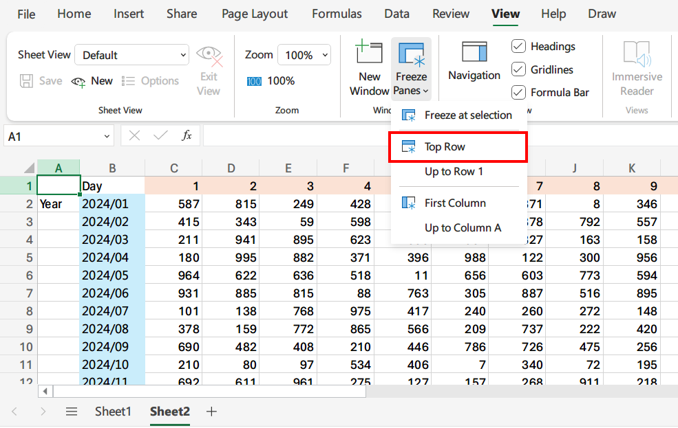
If we want to freeze the top row, just move the active cell to A1 and use the Ribbon menu (shown below): View → Freeze Panes → Top Row

Occassionally, we need to compare other rows with the second row, for example row 20 with row 2. Under this circumstance, we can freeze the top TWO rows.

Freezing the top two rows can be achieved as follows.

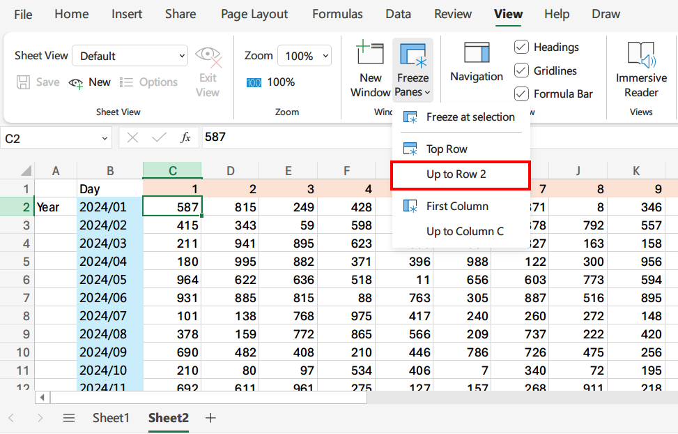
Step 1: Place the active cell at A2 (or any other cell in the second row)

Step 2: Use the Ribbon menu (shown below): View → Freeze Panes → Top Row

After freezing the top two rows, we can now compare the data of row 2 and row 20 side by side just like the next screenshot.

Freeze the column

Just like the way of freezing the row, we can also freeze a column in an Excel worksheet.

Suppose we wanna freeze the first column, just move the active cell to A1 and use the Ribbon menu (shown below): View → Freeze Panes → Top Row

Similarly, we can freeze multiple columns together.

Freezing the first two columns (column A and column B) can be configured as below.

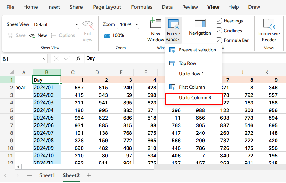
Step 1: Place the active cell at B1 (or any other cell in the second column)

Step 2: Use the Ribbon menu: View → Freeze Panes → Up to Column B

Freeze both the row and the column at the same time

Once in a while we will encounter a situation in which both the row and column have to be freezed.

No problem. Just follow the illustrations below.

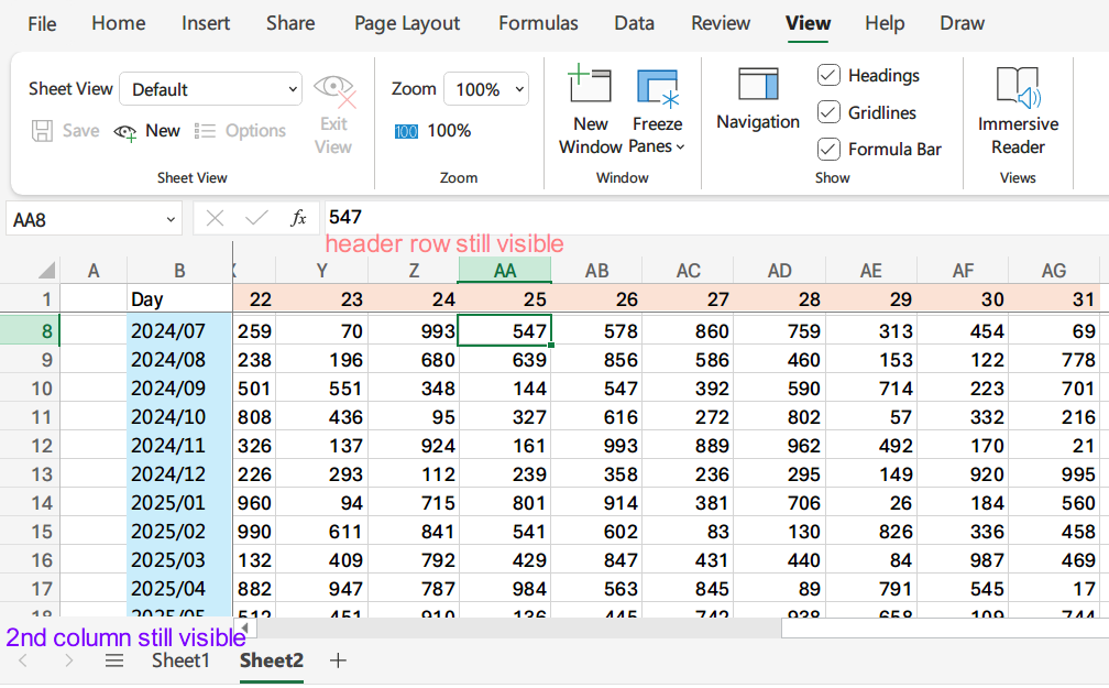
Assume that we have to freeze both the first row AND the first two columns (column A and B).

Step 1: Place the active cell exactly at C2 (Caveat: this location is a must.)

Step 2: Use the Ribbon menu: View → Freeze Panes → Freeze at selection

After performing this freezing, we can scroll the worksheet AND still have the header row (light orange background) and the first two columns remain visible as we scroll as the following image.

After reading this article, hopefully next time when you need to freeze rows or columns in Excel online, NO MORE FREEZING in not knowing what to do. 🙂